Credit risk analysis provides lenders with a complete profile of the customer and an insight that enables them to understand customer behaviour.

New Methods

Today, advanced analytics techniques enable firms to analyse the risk level for those clients with little to no credit account based on data points. Let’s list down the methods used for credit risk analysis.

Standard Deviation

In this method, formula measures the dispersion of data from its expected value. The standard deviation is employed in making an investment decision to measure the amount of historical volatility compared with an investment relative to its annual rate of return. It indicates how much the current return is diverging from its supposed historical normal returns. For example, a stock that has a high standard deviation experience larger volatility, and accordingly, a higher level of risk is compared with the stock.

Beta Measure

Beta is another popular measure of risk. Beta measures the volume of systematic risk individual security or an industrial sector has related to the whole stock market. The market has a beta of 1, and it can be practised to gauge the risk of security. If a security’s beta is equivalent to 1, the security’s price moves in time step with the market. A security with a beta higher than 1 indicates that it is more volatile than the market. Conversely, if a security’s beta is smaller than 1, it symbolises that the security is less volatile than the market. For example, assume a security’s beta is 1.5. In hypothesis, the security is 50 per cent more volatile than the market.

Value At Risk(VAR)

VAR is a statistical model used to estimate the level of risk connected with a portfolio or company. VaR estimates the maximum potential decline with a degree of reliance for a specified period. For illustration, assume a portfolio of investments has a one-year 10 per cent VAR of $5 million. Consequently, the portfolio has a 10 per cent probability of losing more than $5 million over a one-year period.

Conditional VAR

It is another risk measure adopted to estimate the tail risk of an investment. Used as an extension to VaR, the conditional VaR estimates the likelihood, with a particular degree of confidence, that there will be a break in the VaR; it seeks to assess what happens to an investment exceeding its maximum loss threshold. This measure is more susceptible to events that happen in the tail end of distribution – the tail risk. For illustration, a risk manager thinks the average loss on an investment is $10 million for the worst 1 per cent of potential outcomes for a portfolio. Therefore, the conditional VaR, or anticipated shortfall, is $10 million for the 1 per cent tail.

Implementing With Python

To calculate Credit Risk using Python we need to import data sets. For example, we take up a data which specifies a person who takes credit by a bank. Each individual is classified as a good or bad credit risk depending on the set of attributes. It’s impossible to understand the original dataset due to its complicated system of categories and symbols. The data set can be converted into a CSV file format which can be understood easily. The following are some of the attributes that are to be mentioned in the data set.

The entire data set for the program is taken from https://archive.ics.uci.edu/ml/datasets/Statlog+%28German+Credit+Data%29

Code and picture credits: https://www.kaggle.com/kabure/predicting-credit-risk-model-pipeline

Age (numeric)

Sex (text: male, female, other)

Job (numeric: 0 – unskilled and non-resident, 1 – unskilled and resident, 2 – skilled, 3 – highly skilled)

Housing (text: own, rent, or free)

Saving accounts (text – little, moderate, quite rich, highly rich)

Checking account (numeric)

Credit amount (numeric, in DM)

Duration (numeric, in the month)

Purpose(text: car, furniture/equipment, radio/TV, domestic tools, repairs, education, enterprise, vacation/others

Risk (Value  – Good or Bad Risk)

Code:

import pandas as pd #Library To work with a dataset
import numpy as np #Math library
import seaborn as sns #Graph library that use matplot in preparation
import matplotlib.pyplot as plt #to plot unusual parameters in seaborn

#Importing the data

df_credit = pd.read_csv(“.######################.”,index_col=0)

print(df_credit.info())

#Looking unique values
print(df_credit.nunique())
#Looking the data
print(df_credit.head())

Format for the plot grid:

[(1,1) x1,y1][(1,2)x2,y2][(2,1)x3,y3]

# Credit Amount column
interval = (18, 25, 35, 60, 120)

cats = [‘Student’, ‘Young’, ‘Adult’, ‘Senior’]
df_credit[“Age_cat”] = pd.cut(df_credit.Age, interval, labels=cats)

df_bad = df_credit[df_credit[“Risk”] == ‘bad’]
df_good = df_credit[df_credit[“Risk”] == ‘good’]

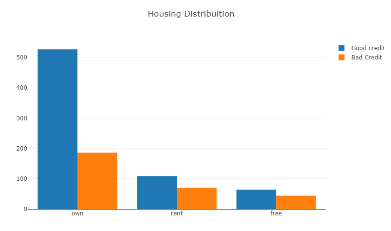
Distribution of Housing own and rent by risk factor

Code:

# 1st plot
trace0 = go.Bar(
x = df_credit[df_credit["Risk"]== 'good']["Housing"].value_counts().index.values,
y = df_credit[df_credit["Risk"]== 'good']["Housing"].value_counts().values,
name='Good credit'
)

2nd plot

trace1 = go.Bar(
x = df_credit[df_credit[“Risk”]== ‘bad’][“Housing”].value_counts().index.values,
y = df_credit[df_credit[“Risk”]== ‘bad’][“Housing”].value_counts().values,
name=”Bad Credit”
)

data = [trace0, trace1]

layout = go.Layout(
title=’Housing Distribution’
)

fig = go.Figure(data=data, layout=layout)

py.iplot(fig, filename=’Housing-Grouped’)

Distribution of Credit Value by Housing

Code:

fig = {
"data": [
{
"type": '###',
"x": df_good['Housing'],
"y": df_good['Credit _amount'],
"legendgroup": 'Good Credit',
"scalegroup": 'No',
"name": 'Good _Credit',
"side": 'negative',
"box": {
"visible": True
},
"meanline": {
"visible": True
},
"line": {
"color": '###'
}
},
{
"type": '###',

“x”: df_bad[‘Housing_’],
“y”: df_bad[‘Credit_amount’],
“legendgroup”: ‘Bad Credit’,
“scalegroup”: ‘No’,
“name”: ‘Bad Credit’,
“side”: ‘positive’,
“box”: {
“visible”: True
},
“meanline”: {
“visible”: True
},
“line”: {
“color”: ‘green’
}
}
],
“layout” : {
“yaxis”: {
“zeroline”: False,
},

“violingap”: 0,
“violinmode”: “over_lay”
}
}

py.iplot(fig, filename = ‘violin_/split’, validate _= False)

In Conclusion

Today, credit risk analysts work across various sectors like Consumer & Retail, Gaming, Healthcare, Insurance, Finance, Media & Telecom, Natural Resources, Banks, Broker and Asset Managers and many more.