In Machine Learning context, there are typically two kinds of learners or algorithms, ones that learn well the correlations and gives out strong predictions and the ones which are lazy and gives out average predictions that are slightly better than random selection or guessing. The algorithms that fall into the former category are referred to as strong learners and the ones that fall into the latter are called weak or lazy learners.

Boosting essentially is an ensemble learning method to boost the performances or efficiency of weak learners to convert them into stronger ones. Boosting simply creates a strong classifier or regressor from a number of weak classifiers or regressors by learning from the incorrect predictions of weak classifiers or regressors.

The Simple  Intuition Behind Boosting

Before we get into boosting, a short reminder to all Data Science folks,  Machinehack has launched the latest hackathon – Predicting The Costs Of Used Cars – Hackathon By Imarticus Learning in partnership with Imarticus Learning. Be sure to check out the hackathon by clicking here. Participate and win exciting prizes.

Now let’s get back to Boosting, From the definition, it clearly states that boosting is an ensemble method which implies that the algorithm makes use of multiple learners or models. There are different ensemble methods to improve the accuracy of predictions over a given dataset, for example, bagging or stacking. However the major difference between bagging and boosting lies in the fact that in bagging the predictions of each model is individually considered and then aggregated to produce a better result while in boosting the different algorithms work closer by learning from each other.

Let us understand with an example:

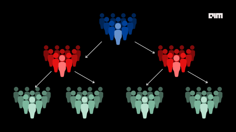
Consider a binary classification problem where we are classifying a group of apples and oranges. Let’s say there are 3 classifiers in the ensemble and there are 3 apples and 3 oranges.

Step 1: The classifier 1 suppose, predicts correctly for 2 of the 3 apples and misclassified one as orange.

Step 2: The second classifier then picks up the wrong prediction from the first classifier and assigns a higher weight to it and generates its own predictions.

Step 3: Step 2 is repeated with the 3rd classifier for wrong predictions and the weights are adjusted.

Step 4: steps 2 and 3 repeats until an optimal result is obtained.

The adaboost classifier can be mathematically expressed as :

Where:

fi is the ith classifier and theta-i is the corresponding weight.

Boosting Algorithms

There have been many boosting algorithms that popped up recently, some of the popular ones being XGBoost, Gradient Boosting, LPBoost, TotalBoost, BrownBoost, LogitBoost etc.

However, the first ever algorithm to be classed as a boosting algorithm was the AdaBoost or Adaptive Boosting, proposed by Freund and Schapire in the year 1996. AdaBoost is a classification boosting algorithm.

Implementing Adaptive Boosting: AdaBoost in Python

Having a basic understanding of Adaptive boosting we will now try to implement it in codes with the classic example of apples vs oranges we used to explain the Support Vector Machines. Click here to download the sample dataset used in the example of AdaBoost in Python below.

Let us begin!

Importing the dataset

import pandas as pd
data = pd.read_csv("apples_and_oranges.csv")

Splitting the dataset into training and test samples

from sklearn.model_selection import train_test_split
training_set, test_set = train_test_split(data, test_size = 0.2, random_state = 1)

Classifying the predictors and target

X_train = training_set.iloc[:,0:2].values
Y_train = training_set.iloc[:,2].values
X_test = test_set.iloc[:,0:2].values
Y_test = test_set.iloc[:,2].values

Initializing Adaboost classifier and fitting the training data

from sklearn.ensemble import AdaBoostClassifier
adaboost = AdaBoostClassifier(n_estimators=100, base_estimator= None,learning_rate=1, random_state = 1)
adaboost.fit(X_train,Y_train)

If we look closer into the above code block we will see an argument called  ‘base_estimator’ which is set to None for the AdaBoostClassifier. By default the AdaBoostClassifier selects Decision Tree classifier as the base classifier or weak learner as in this case. We can also specify other classifiers provided it that must support the calculation of class probabilities.

Predicting the classes for test set

Y_pred = adaboost.predict(X_test)

Attaching the predictions to test set for comparing

test_set["Predictions"] = Y_pred

Comparing the actual classes and predictions

We can see that the predictions are identical to the actual observations which imply a test accuracy of 100%.

Calculating the accuracy of the predictions:

from sklearn.metrics import confusion_matrix
cm = confusion_matrix(Y_test,Y_pred)
accuracy = float(cm.diagonal().sum())/len(Y_test)
print("\nAccuracy Of AdaBoost For The Given Dataset : '', accuracy)

Output:

Accuracy Of AdaBoost For The Given Dataset: 1.0

Visualizing the predictions

Before we visualize we need to encode the classes ‘apple’ and ‘orange’ into numerals. We can achieve that using the label encoder.

#Encoding
from sklearn.preprocessing import LabelEncoder
le = LabelEncoder()
Y_train = le.fit_transform(Y_train)

#Fitting the encoded data to AdaBoostClassifier
from sklearn.ensemble import AdaBoostClassifier
adaboost = AdaBoostClassifier(n_estimators=100, base_estimator= None,learning_rate=1, random_state = 1)
adaboost.fit(X_train,Y_train)

#Visualising
import numpy as np
import matplotlib.pyplot as plt
from matplotlib.colors import ListedColormap
plt.figure(figsize = (7,7))
X_set, y_set = X_test, Y_test
X1, X2 = np.meshgrid(np.arange(start = X_set[:, 0].min() - 1, stop = X_set[:, 0].max() + 1, step = 0.01),
np.arange(start = X_set[:, 1].min() - 1, stop = X_set[:, 1].max() + 1, step = 0.01))
plt.contourf(X1, X2, adaboost.predict(np.array([X1.ravel(), X2.ravel()]).T).reshape(X1.shape),
alpha = 0.75, cmap = ListedColormap(('black', 'white')))
plt.xlim(X1.min(), X1.max())
plt.ylim(X2.min(), X2.max())

for i, j in enumerate(np.unique(y_set)):
plt.scatter(X_set[y_set == j, 0], X_set[y_set == j, 1],
c = ListedColormap(('red', 'orange'))(i), label = j)

plt.title('Apples Vs Oranges Predictions')
plt.xlabel('Weight In Grams')
plt.ylabel('Size in cm')
plt.legend()
plt.show()

Output:

On comparing with the results of SVM classifier that we saw in the article – Understanding The Basics Of SVM With Example And Python Implementation which attained an accuracy of 0.875 or 87% we can see that AdaBoost has predicted with the perfection on all the classes with a 100% accuracy on the given data.

Also, be sure to check out our tutorial for implementing Gradientboosting and XGBoost.