Dimensionality Reduction is an important and necessary step when we have big data in hand with so many features. When there are so many features or columns, it is hard to understand the correlation between them. Including weak links or correlations in training-data can also result in an inaccurate prediction by the model.  Dimensionality Reduction takes care of this situation by removing unnecessary features thus helping in fitting the model with the right and most relevant features.

Principal Component Analysis is one of the most sought after Dimensionality Reduction techniques in Machine Learning. In one of our previous articles, we saw how PCA can be implemented in Python.

In this article, we will learn to implement the PCA in R programming. Readers are expected to have some familiarity with the programming language.

Here are some good reads on Dimensionality Reduction :

• Understanding Dimensionality Reduction Techniques To Filter Out Noisy Data
• Introduction to DimensionalityReduction
• A Hands-On Guide To Dimensionality Reduction

For implementing PCA in R we will use the How To Choose The Perfect Beer dataset from MachineHack. To get the dataset head to MachneHack, sign up and download the datasets from the Attachment Section.

Having trouble finding the data set? Click here to go through the tutorial to help yourself.

Lets Code!

Importing the Dataset

We will be using a smaller subset of the original dataset and it has been preprocessed to some extent. To know more about processing please check out Data Preprocessing With R: Hands-On Tutorial.

dataset = read.csv('Beer_dataset.csv')

The Dataset is as shown below :

Creating Training set and Test set

library(caTools)
set.seed(123)
split = sample.split(dataset$Score, SplitRatio = 0.80)
training_set = subset(dataset, split == TRUE)
test_set = subset(dataset, split == FALSE)

After executing the above code block, we will get two distinct dataframes, the training_set and the test_set.

Without further Preprocessing we will directly fit the model to a Linear Regressor

Initialising the Model and Fitting the Training Data:

# Multiple Linear Regressor
mlr = lm(formula = Score ~ . , data = training_set )
print(mlr)
Output:

Predicting for the Test Set

predy = predict(mlr, newdata = test_set)

This code block will result in an array consisting of the predictions.

Evaluating The Performance

actuals_and_preds <- data.frame(cbind(actuals=test_set$Score, predicteds = predy))

The above code block will result in a dataframe consisting of the predictions and the true or actual test data.

Output :

To evaluate we will consider a more basic MIN-MAX Accuracy.

min_max_accuracy <- mean(apply(actuals_and_preds, 1, min) / apply(actuals_and_preds, 1, max))print(min_max_accuracy)

Output:

0.7055808

Implementing PCA

Importing Necessary Libraries

install.packages("caret") # Execute Once
library(caret)
install.packages("e1071") # Execute Once
library(e1071)

Initializing PCA And Fitting Data

pca = preProcess(training_set[-9], method = 'pca', pcaComp = 2)

The above code block initializes a pca object and fits the training data. The parameter pcaComp refers to the number of principal components you want the model to return. Here the model will return 2 Principal Components.

Generating the Principal Components

training_set.pca = predict(pca, training_set)
test_set.pca = predict(pca, test_set)

This code block will create two new data sets with only the Principal Components and the Actual dependent factor (Score) as columns/features.

Reordering the Columns

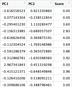
training_set.pca = training_set.pca[c(2,3,1)]
test_set.pca = test_set.pca[c(2,3,1)]

Output:

training_set.pca:

test_set.pca:

Using Linear Regression to Predict From The Principal Components

mlr_pca = lm(formula = Score ~ . , data = training_set.pca)print(mlr_pca)

Output:

Predicting With The Principal Components

predy_pca = predict( mlr_pca, newdata = test_set.pca)

Measuring The Accuracy

actuals_and_preds_pca <- data.frame(cbind(actuals= test_set.pca$Score, predicteds = predy_pca))

min_max_accuracy_pca <- mean(apply(actuals_and_preds_pca, 1, min) / apply(actuals_and_preds_pca, 1, max))print(min_max_accuracy_pca)
Output

0.7301324

Conclusion

Comparing the accuracies from the Linear Regression Models, we can see a slight improvement in the accuracy in the model that was fitted with the principal components. The model actually improved with only two features predicting as compared to the original dataset’s 8 independent features. Thus Dimensionality Reduction with PCA holds a significant role in Data Science especially considering the vastness of the data sets that needs to be processed.