Time Series data is one of the most common types of data that is available today. The data can be about how a person’s salary changes over the years, it can be about how the value of INR compares to other currencies over a period of time — everything that changes with time forms Time-Series. 

In this article, we will understand what is Time-Series Forecasting and will look into some basic terminologies we use while performing a Time-Series Analysis.

What Is Time-Series Forecasting

Time Series Analysis and Forecasting is the process of understanding and exploring Time Series data to predict or forecast values for any given time interval. This forms the basis for many real-world applications such as Sales Forecasting, Stock-Market prediction, Weather forecasting and many more.

Not all data that has timestamps or Dates as its feature or column can be considered as a Time Series data. A time-series data should consist of observations over a regular and continuous interval.

Here are some examples of Time Series Data:

• Records of observations of daily stock-price from the start of the year to the end of the year.
• The hourly observation of rise and fall in Bitcoin price over a period of time. 

Given below is an example dataset that consists of the daily opening and closing price of Bitcoin.

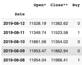
 Univariate vs Multivariate Time Series

When there is only a single variable that can be used to determine its value for an unknown interval of time, it is called a Univariate Time Series. When there is more than one independent variable that determines the values of the dependent variable over unknown intervals of time, it is called a Multivariate Time Series. The image shown above is an example of Multivariate Time Series.

Time Series Patterns

When dealing with large Time Series datasets, there are certain patterns that one would come across. Time Series data may have the following patterns.

• Trend: Trend can be  a linear or nonlinear component and its value may either decrease or increase with respect to time by changing its directions
• Seasonal: A  linear or nonlinear pattern that repeats at particular intervals. Seasonality is a very common feature or characteristics of Sales data
• Cyclic: It is a wave-like pattern that persists over a longer period. Cycles are often irregular and mostly appears in combination with other patterns
• Random/Noise: A random component that does not have or follow a specific pattern

Stationarity

In Time Series Analysis, stationarity is a characteristic property of having constant statistical measures such as mean, variance, co-variance etc over a period of time. In other words, a Time-Series is said to be stationary if the marginal distribution of y at a time p(yt) is the same at any other point in time. For Time Series Analysis to be performed on a dataset, it should be stationary. 

Given below is an example of Non-Stationary data.

Popular Models For Solving Time Series

AutoRegressive Model

Auto-Regressive Model popularly known as the AR model is one of the simplest models for solving Time Series. The value of y at time t depends on the value of y at time t-1. If y depends on more than one of its previous values then it is denoted by p parameters.

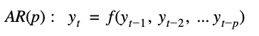
Where p is the number of past values to consider.

Moving Average Model

While the autoregressive model considered the past values of the target variable for prediction, Moving average makes use of the white noise error terms.

It can be represented as follows:

Where,

εt, εt−1,…, εt−q are the white noise error terms.

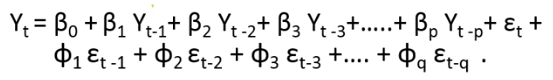
ARMA

The Autoregressive Moving Average model is a combination of the Autoregressive model and the moving average model which uses both the past values as well as the error terms to predict for future time series.

ARMA can be Mathematically expressed as follows:

ARIMA

Autoregressive Integrated Moving Average is a very popular model used in Time-Series forecasting. The model is a generalization of the ARMA model that uses integration for attaining stationarity.

The ARIMA model makes use of 3 parameters as given below:

p: Lag order or the number of past orders to be included in the model

d: The degree of differentiation to be applied.

q: The order of moving average.

Outlook

Time Series Forecasting is an integral part of Machine Learning that evaluates and understands the time series data to predict future outcomes. It has wide applications in Banking, Finance, Weather Forecasting and Sales Forecasting among others.